topic badge
United States of AmericaVA
Algebra, Functions, and Data Analysis

3.02 Z-scores

Z-scores

To directly compare multiple normally distributed data sets, we need a common unit of measurement. In statistics involving the normal distribution, we use the number of standard deviations away from the mean as a standardized unit of measurement called a z-score.

z-score

The number of standard deviations an element is away from the mean.z=\dfrac{x-\mu}{\sigma} where x is an element of the data set, \mu is the mean of the data set, and \sigma is the standard deviation of the data set.

Exploration

Imagine two students took different standardized tests. Student A scored 1200 on the SAT, where the mean was 1050 and the standard deviation was 200. Student B scored 25 on the ACT, where the mean was 21 and the standard deviation was 5.

  1. How far above the mean did Student A score on the SAT?

  2. How far above the mean did Student B score on the ACT?

  3. Based only on the distance above the mean, who seems to have performed better?

  4. Now consider the spread (standard deviation) of the scores. How many standard deviations above the mean was Student A's score? How many standard deviations above the mean was Student B's score?

  5. Thinking about performance relative to others taking the same test (i.e., considering standard deviations), who performed better? Why is just looking at the raw score difference from the mean potentially misleading when comparing scores from different distributions?

We can use z-scores along with the standard normal distribution to compare values from different sets of data.

The standard normal distribution

A specific normal distribution with a mean of 0 and a standard deviation of 1. It represents the distribution of all possible z-scores.

Standardizing data using z-scores transforms any normal distribution into the standard normal distribution, which allows for the comparison of unlike normal data.

A standard normal distribution curve, which is bell-shaped and symmetric. The horizontal axis is centered at the mean, 0. The standard deviation is 1.

For example, a data set that is normally distributed with a mean of 1010 and a standard deviation of 20 can be standardized with z-scores. This would allow us to compare other sets of similar data with a different mean and standard deviation.

Two curves. The left curve is titled A Normal Distribution, with a mean of 1,010. A right arrow labeled Standardize is pointing from the left curve to the right curve. The right curve is titled The Standard Normal Distribution, with a mean of 0. Speak to your teacher for more details.

To find the z-score of a data value, we must know the mean and standard deviation. If we know those values, we can use the following formula to find the equivalent z-score.

\displaystyle z=\dfrac{x-\mu}{\sigma}
\bm{z}
The z-score
\bm{x}
The data value
\bm{\mu}
The population mean
\bm{\sigma}
The population standard deviation
  • A positive z-score indicates the data value was above the mean.

  • A z-score of 0 indicates the data value was equal to the mean.

  • A negative z-score indicates the data value was below the mean.

  • The larger the magnitude of the z-score, the further the score is from the mean.

The empirical rule can also be used to estimate the percentage of data within 1, 2, and 3 standard deviations on the mean in the standard normal distribution.

A normal distribution curve. Below the curve is a horizontal axis with the following evenly spaced marks from left to right:-3, -2, -1, 0, 1, 2, 3. The peak of the curve is at 0. Vertical lines are drawn from the curve to each mark in the horizontal axis. The area under the curve between -3 and -2 is labeled 2.35%, between -2 and -1 labeled 13.5%, between -1 and 0 labeled 34%, between 0 and 1 labeled 34%, between 1 and 2 labeled 13.5%, and between 2 and 3 labeled 2.35%. Below the horizontal axis, a set of three brackets are shown: a bracket connecting -1 and 1 is labeled 68%, a bracket connecting -2 and 2 is labeled 95%, and a bracket connecting -3 and 3 is labeled 99.7%.

Examples

Example 1

Brock is applying to different colleges across America and needs to decide if he should emphasize his SAT score, ACT score, or both. The test scores for both the SAT and ACT are normally distributed. The data is summarized in the table.

Brock's scoreMeanStandard Deviation
SAT14501051211
ACT3020.85.7
a

Calculate and interpret the z-score for Brock's SAT score.

Worked Solution
Create a strategy

The formula for finding the z-score is z=\dfrac{x-\mu}{\sigma}, where x is a test score, \mu is the mean, and \sigma is the standard deviation.

Apply the idea

For the SAT, we are given x=1450, \mu=1051, and \sigma=211:

\displaystyle z\displaystyle =\displaystyle \dfrac{x-\mu}{\sigma}Formula for z-scores
\displaystyle z\displaystyle =\displaystyle \dfrac{1450-1051}{211}Substitute the known values
\displaystyle z\displaystyle \approx\displaystyle 1.89Evaluate

Brock's z-score for his SAT test is z \approx 1.89, which means Brock scored approximately 1.89 standard deviations above the mean.

b

Calculate and interpret the z-score for Brock's ACT score.

Worked Solution
Create a strategy

We will use the formula for z-scores again, but this time with the given values for the ACT.

Apply the idea

For the ACT, we are given x=30, \mu=20.8, and \sigma=5.7:

\displaystyle z\displaystyle =\displaystyle \dfrac{x-\mu}{\sigma}Formula for z-scores
\displaystyle z\displaystyle =\displaystyle \dfrac{30-20.8}{5.7}Substitute the known values
\displaystyle z\displaystyle \approx\displaystyle 1.61Evaluate

Brock's z-score for his ACT test is z\approx 1.61, which means Brock scored approximately 1.61 standard deviations above the mean.

c

Determine which test Brock did better on relative to all other SAT and ACT test takers.

Worked Solution
Create a strategy

Compare the z-scores found in parts (a) and (b). The higher Brock's z-score, the better he did relative to the other test takers.

Apply the idea

Relative to all people who took the SAT and ACT, Brock did slightly better on his SAT test than he did on his ACT test since his z-score was higher.

Reflect and check

Both of Brock's scores were better than average, but similar relative to the averages, so he can report either of the test scores when applying to different colleges. On college applications, only one test score is usually required.

Example 2

Three sprinters are training for a national competition. The data collected on each of their running times (in seconds) is approximately normal. Information for their mean, standard deviation, a practice 400\text{ m} sprint and its corresponding z-score are in the table.

\mu\sigmaz\text{-score}\text{Practice time}
Lina653-1.27
Aurelia620.8565.4
Mariana2-0.559.5
a

Find the 400\text{ m} sprint time Lina ran during practice.

Worked Solution
Create a strategy

To find the practice time that had a z-score of -1.27, we can use the formula z=\dfrac{x-\mu}{\sigma} with the given mean, standard deviation, and z-score, then solve for the practice time in seconds.

Apply the idea

From the given information, we know \mu=65, \sigma=3, and z=-1.27.

\displaystyle z\displaystyle =\displaystyle \dfrac{x-\mu}{\sigma}Formula for z-scores
\displaystyle -1.27\displaystyle =\displaystyle \dfrac{x-65}{3}Substitute known values
\displaystyle -3.81\displaystyle =\displaystyle x-65Multiply both sides by 3
\displaystyle 61.19\displaystyle =\displaystyle xAdd 65 to both sides

Lina ran a 400\text{ m} practice time of 61.19 seconds.

Reflect and check

Running a 400\text{ m} race in 61.19 seconds is -1.27 standard deviations below the sprinter's average time of 65 seconds. This tells us she ran faster in that practice run than she normally does.

b

Find the standard deviation of Aurelia's times.

Worked Solution
Create a strategy

To find the standard deviation, we can use the z-score formula with the given mean, z-score, and practice time, then solve for the standard deviation.

Apply the idea

From the given information, we know \mu=62, z=0.85, and x=65.4.

\displaystyle z\displaystyle =\displaystyle \dfrac{x-\mu}{\sigma}Formula for z-scores
\displaystyle 0.85\displaystyle =\displaystyle \dfrac{65.4-62}{\sigma}Substitute known values
\displaystyle 0.85\displaystyle =\displaystyle \dfrac{3.4}{\sigma}Evaluate the numerator
\displaystyle 0.85\sigma\displaystyle =\displaystyle 3.4Multiply both sides by \sigma
\displaystyle \sigma\displaystyle =\displaystyle 4Divide both sides by 0.85

Aurelia's 400\text{ m} times have a standard deviation of 4 seconds.

c

Find the average 400\text{ m} sprint time for Mariana.

Worked Solution
Create a strategy

To find the mean, we can use the z-score formula with the given standard deviation, z-score, and practice time, then solve for the mean.

Apply the idea

From the given information, we know \sigma=2, z=-0.5, and x=59.5.

\displaystyle z\displaystyle =\displaystyle \dfrac{x-\mu}{\sigma}Formula for z-scores
\displaystyle -0.5\displaystyle =\displaystyle \dfrac{59.5-\mu}{2}Substitute known values
\displaystyle -1\displaystyle =\displaystyle 59.5-\muMultiply both sides by 2
\displaystyle -60.5\displaystyle =\displaystyle -\muSubtract 59.5 from both sides
\displaystyle 60.5\displaystyle =\displaystyle \muMultiply both sides by -1

Mariana's average 400\text{ m} time is 60.5 seconds.

Reflect and check

Of the three sprinters, Mariana has the fastest average 400\text{ m} time, and her sprint times are more consistent.

Example 3

An extreme amusement park ride only allows riders over 60 inches tall to ride. Colette was not allowed to ride because she did not meet the height requirement, but her younger brother Gavin was able to ride because he was taller than the height requirement. This led her to ask the question, "How do the heights of men compare to the heights of women?"

a

Describe a method Colette can use to collect data.

Worked Solution
Create a strategy

To eventually compare heights using z-scores, we first need a method for gathering the raw data. Consider Colette's statistical question and the practical ways to collect information about people's heights.

Then, consider whether the data can be collected by research, a survey, an observation, or a scientific experiment.

Apply the idea

Colette needs to collect data on the heights of men and women. Since most people know their heights, Colette can use a survey or poll to collect the data.

Reflect and check

Colette could also research the average heights of men and women. While researching, she would need to make sure that the sample is representative of the population, and the data collection process did not introduce bias.

b

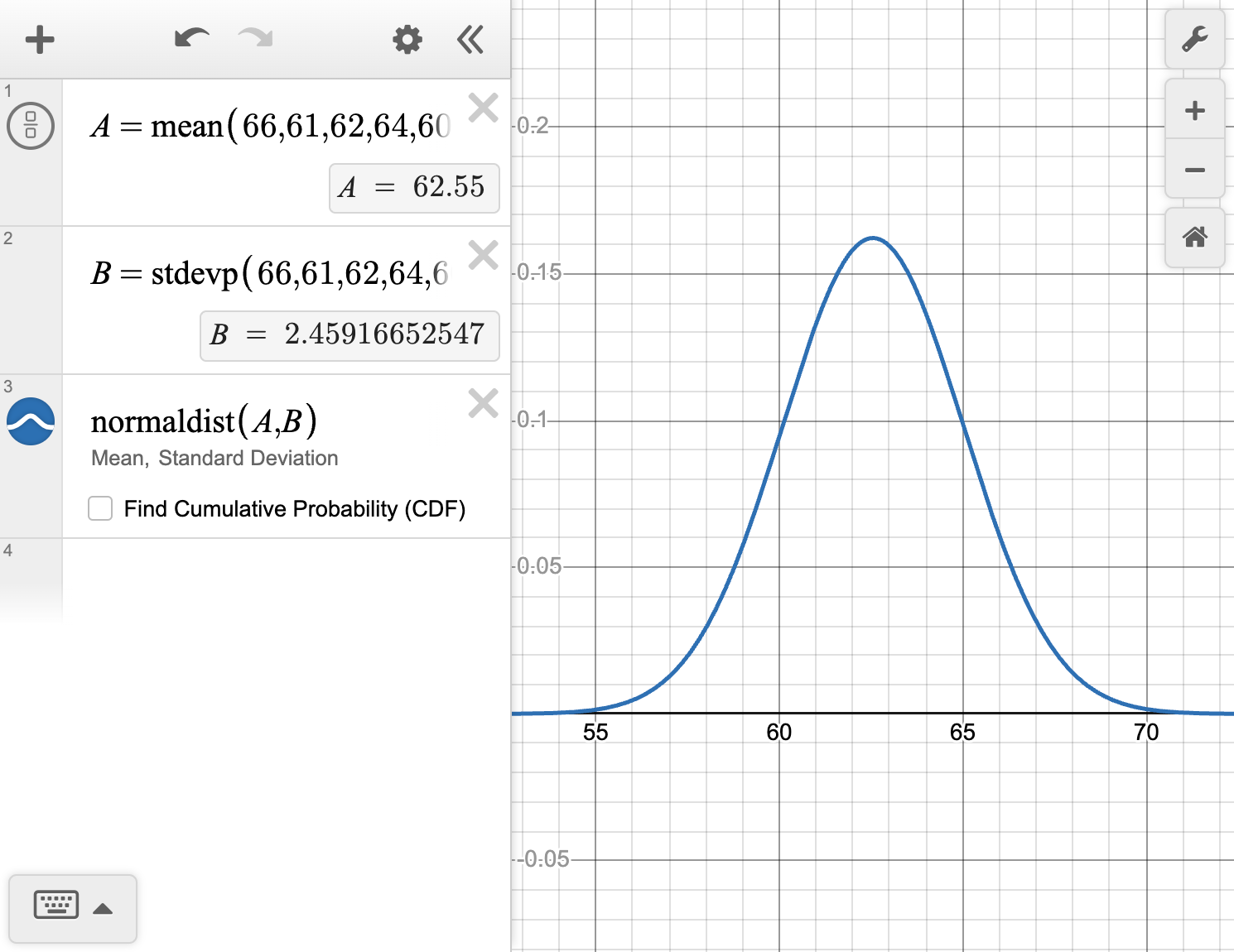
The data Colette collected on the heights of men and women is in the table.

Female heightsMale heights
66, 61, 62, 64, 60,\\62, 64, 63, 58, 64,\\60, 68, 62, 59, 64,\\60, 64, 66, 62, 6271, 69, 71, 66, 69,\\77, 74, 72, 75, 71,\\68, 72, 70, 64, 73,\\68, 66, 70, 67, 73

Use technology to create a smooth curve to model each distribution and describe the shape of each curve.

Worked Solution
Create a strategy

Before calculating z-scores, we need to understand the shape of the distributions and find their mean and standard deviation. Technology can help visualize the data and calculate these key statistics.

Using the Desmos graphing calculator, we can follow these steps to create a smooth curve of the data:

  1. Find the mean of the data using the built-in \text{mean} function.

  2. Find the population standard deviation of the data using the built-in \text{stdevp} function.

  3. Create the smooth curve using the built-in \text{normaldist} function.

  4. Click the magnifying glass with the plus sign to see the curve.

Apply the idea

First, we will create the smooth curve that approximates the women's heights.

A screenshot of the Desmos graphing calculator. A list of data points for female heights is entered. The commands mean(F), stdevp(F), and normaldist(mean(F), stdevp(F)) are used to calculate statistics and plot the normal distribution curve for the data. Speak to your teacher for more details.

The curve is symmetric and bell-shaped, meaning the data is approximately normal.

Next, we will create the smooth curve that approximates the men's heights.

A screenshot of the Desmos graphing calculator. A list of data points for male heights is entered. The commands mean(M), stdevp(M), and normaldist(mean(M), stdevp(M)) are used to calculate statistics and plot the normal distribution curve for the data. Speak to your teacher for more details.

Again, the curve is symmetric and bell-shaped, meaning the data is approximately normal.

Reflect and check

Although both data sets are normally distributed, they have different measures of center and spread. This means the curves will have a similar shape, but one is likely taller than the other and they are centered around different values.

A screenshot of the Desmos graphing calculator showing the normal distribution curves for two data sets, female heights and male heights, plotted on the same axes. The curve for male heights is shifted to the right of the curve for female heights. Speak to your teacher for more details.
c

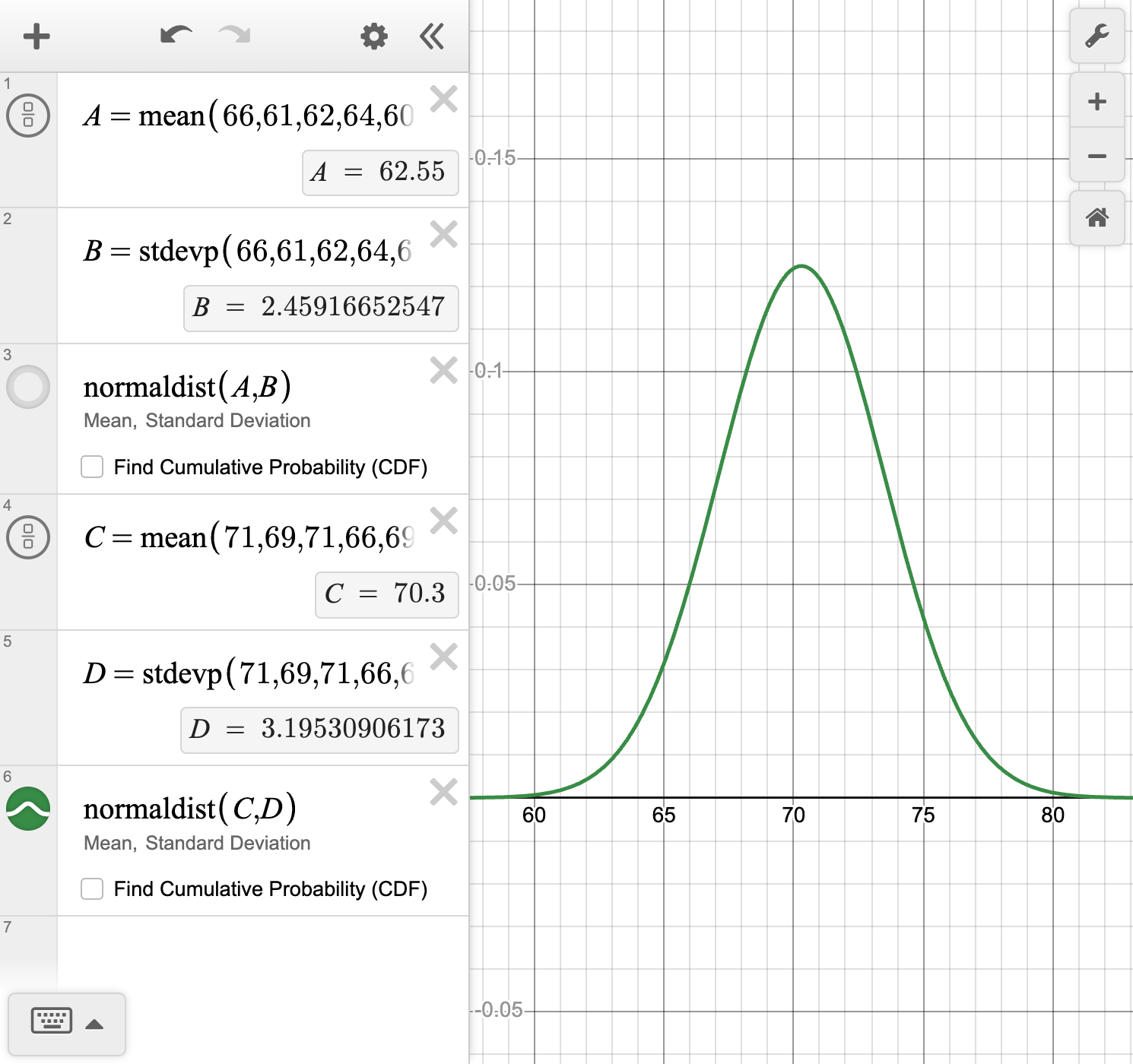
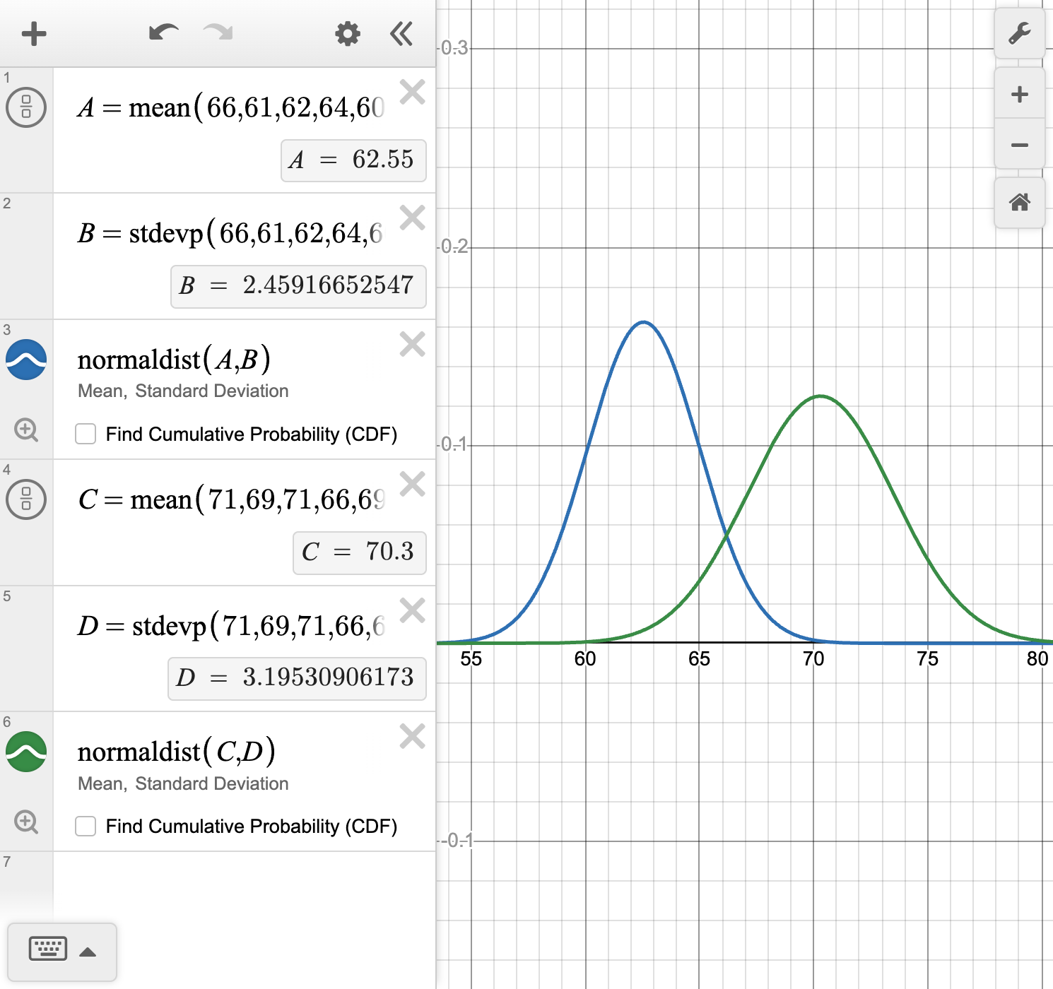
Answer the statistical question that Colette formulated.

Worked Solution
Create a strategy

Colette's initial question asks for a direct comparison of typical heights. Using the means calculated in the previous step provides a direct answer to this preliminary question, setting the stage for the z-score comparison related to the ride requirement.

Apply the idea

Looking at the smooth curves from the previous part, we can see that the curve that approximates the women's heights is centered at around 63 inches. The curve that approximates the men's heights is centered at 70 inches.

This tells us that, on average, men are taller than women.

Reflect and check

Rather than using the curves to compare the means, we could have compared the values of the means of each data set, which were also found in the previous part with technology. The mean of the women's heights is 62.55, and the mean of the men's heights is 70.3, showing men are taller on average.

d

Since both data sets are normally distributed, Colette wanted to further investigate men's and women's heights relative to the height requirement for the ride. Her new statistical question is, "How does the percentage of male riders who can ride this ride compare to the percentage of female riders who can ride?"

Find and interpret the z-scores for the 60-inch height requirement relative to the average American female heights and average American male heights.

Worked Solution
Create a strategy

The average height of men and women are different, and the standard deviations of the heights are different as well. We can compare the heights of men and women by using z-scores to standardize the measurements.

To find the z-score, we can use the formula z=\dfrac{x-\mu}{\sigma} with the given height requirement. Then, we can use technology to find the mean and standard deviation of each set.

Apply the idea

In part (b), we calculated the mean and standard deviation for each set of data.

A screenshot of the Desmos graphing calculator showing the normal distribution curves for two data sets, female heights and male heights, plotted on the same axes. The curve for male heights is shifted to the right of the curve for female heights. Speak to your teacher for more details.

For the female data, we see \mu\approx 62.5, \sigma\approx 2.5, and we were given x=60.

We use these rounded values for mean and standard deviation calculated using technology in part (b).

This simplifies calculations and interpretation, especially when relating results to the empirical rule later.

The z-score for women's height is z=\dfrac{60-62.5}{2.5}=-1.

For women, the height restriction of 60 inches is only 1 standard deviation below the average female height.

Next, we will find the mean and standard deviation of men's heights.

For the male data, we see \mu\approx 70, and \sigma\approx 3.

Again, we use the rounded mean and standard deviation found using technology.

The z-score is z=\dfrac{60-70}{3}\approx -3.33.

The height restriction of 60 inches is more than 3 standard deviations below the average male height.

Reflect and check

Notice that the mean and standard deviations of the sets were rounded to use "nice" values. This allows us to sketch the curves more easily. However, we should not round to "nice" values if the difference is relatively large.

We can use the normal distribution curves of the data to check our answers.

Two normal distribution curves are plotted on the same horizontal axis. The first curve, labeled Women's heights, has a mean of 62.5 and standard deviations marked at 60, 65, and 67.5. The second curve, labeled Men's heights, has a mean of 70 and standard deviations marked at 67, 73, and 76. A vertical line at x=60 indicates the height requirement.

The data value of 60 does lie 1 standard deviation below the mean of the women's heights and 3\frac{1}{3} standard deviations below the mean of the men's heights.

e

Compare the percentage of male riders who can ride this ride to the percentage of female riders who can ride.

Worked Solution
Create a strategy

Because we have the z-scores, we can graph the position of the height requirement relative to the men's heights and the women's heights on the same standard normal curve. Then we can use the empirical rule to find and compare the percentages.

A normal distribution curve. Below the curve is a horizontal axis with the following evenly spaced marks from left to right:-3, -2, -1, 0, 1, 2, 3. The peak of the curve is at 0. Vertical lines are drawn from the curve to each mark in the horizontal axis. The area under the curve between -3 and -2 is labeled 2.35%, between -2 and -1 labeled 13.5%, between -1 and 0 labeled 34%, between 0 and 1 labeled 34%, between 1 and 2 labeled 13.5%, and between 2 and 3 labeled 2.35%. Below the horizontal axis, a set of three brackets are shown: a bracket connecting -1 and 1 is labeled 68%, a bracket connecting -2 and 2 is labeled 95%, and a bracket connecting -3 and 3 is labeled 99.7%.
Apply the idea
A standard normal curve. The y-axis is labeled 'Probability density' and the x-axis is labeled 'z-score' from -3 to 3. An arrow labeled 'men z = -3.33' points to a location on the x-axis to the left of -3. Another arrow labeled 'women z = -1' points to the -1 mark on the x-axis.

Using the empirical rule, we can estimate that more than 99.85\% of men will be able to ride this ride. However, only 84\% of women will be able to ride.

Idea summary

Data that is normally distributed can be normalized using z-scores. This allows us to compare data sets that have different means and standard deviations.

To find the z-score of a data value, we must know the mean and standard deviation. If we know those values, we can use the following formula to find the equivalent z-score.

\displaystyle z=\dfrac{x-\mu}{\sigma}
\bm{z}
The z-score
\bm{x}
The data value
\bm{\mu}
The population mean
\bm{\sigma}
The population standard deviation

Remember that a positive z-score means the data value is above the mean, a negative z-score means it's below the mean, and a z-score of 0 means it's equal to the mean. The larger the absolute value of the z-score, the further the data value is from the mean.

Outcomes

AFDA.DA.4d

Calculate and interpret the z-score for a data point, given the mean and the standard deviation.

AFDA.DA.4e

Compare two sets of normally distributed data using a standard normal distribution and z-scores, given the mean and the standard deviation.

AFDA.DA.4h

Investigate, represent, and determine relationships between a normally distributed data set and its descriptive statistics.

What is Mathspace

About Mathspace